Application diagnostics is used to perform in-depth runtime profiling of individual application instances, helping you quickly locate performance bottlenecks at the resource level, such as CPU, memory, threads, and GC. Leveraging the enhanced probe's capability to automatically collect runtime data, users can enable diagnostic capabilities by simply integrating the application, without the need to modify business code.
Prerequisites
Application Type
Access Requirements
Supported Diagnostic Capabilities
Java
Access Solution: Use the Tencent Cloud enhanced Java agent for access. The agent version must be 2.3-20250131 or later.
JDK Version: JDK versions earlier than Java 8u352 are not recommended, as they may pose a memory crash risk.
Operating System: Linux (x64, arm64) and macOS.
Runtime Environment: OpenJDK or another JDK developed based on the HotSpot JVM must be installed. Environments with only a JRE installed are not supported.
Image: Alpine images are not recommended. The JDK included in Alpine images is typically a slim version and may lack the JDK debugging symbols (the binary file $JAVA_HOME/lib/server/libjvm.so), which can cause memory collection to fail.
3. In the filter at the top of the page, select the target region, business system, and application.
4. In the instance list on the left side of the page, select the target instance.
5. Select the diagnostic capability via the tab on the right side of the page.
JVM Analysis
JVM Analysis includes the following charts:
Function
Description
CPU utilization
Displays the trend of CPU usage of JVM processes. CPU utilization is calculated based on the CPU processing time occupied by the JVM.
Heap memory utilization
Displays the trend of Heap memory usage of JVM processes. Memory utilization = actually used memory / maximum memory requested by the JVM from the operating system.
GC count
Displays the trend of the number of GCs per minute for JVM processes.
Average GC time
Displays the trend of GC duration for JVM processes.
Heap memory details
Displays the trend of Heap memory usage of JVM processes.
Non-Heap memory details
Displays the trend of Non-Heap memory usage of JVM processes.
Thread state statistics
Counts the trend of JVM thread quantity based on different thread states.
Thread overview statistics
Counts the trend of JVM thread quantity based on different thread types.
Buffer memory details
Displays the trend of buffer memory usage of JVM processes.
Performance Profiling 2.0
Performance profiling capability directly outputs performance optimization suggestions through the intelligent analysis engine and provides powerful visualization analysis tools such as the enhanced flame graph, helping users quickly locate application performance bottlenecks. Performance profiling currently supports Java and Go applications. The performance profiling capability for Java applications is implemented based on async-profiler technology, while that for Go applications is implemented based on pprof technology. The Tencent Cloud enhanced OpenTelemetry Java Agent and the Tencent Cloud OpenTelemetry-Go Agent have built-in performance profiling capability, which does not rely on any other components and can collect profiling data with minimal performance overhead.
Creating a Collection Task
1. Click Create Collection Task.
2. In the pop-up dialog box, adjust options such as the collection type as needed, and then click Confirm.
Option Name
Description
Collection Type
Currently supports two collection types: CPU sampling analysis and memory sampling analysis.
CPU Sampling Analysis: Profiles code blocks based on their execution time on the CPU.
Memory Sampling Analysis: Profiles based on memory usage.
Sampling Duration
Sampling duration represents the time length for each profiling data collection. The actual collection time is slightly longer than the sampling duration.
Target Time
Target time represents the execution time of the first profiling after the profiling task is created.
Execute Now: Perform profiling without waiting.
Specified Time: Specify any time point within the next 24 hours to execute profiling.
Execution Count
Number of executions represents how many times a profiling task will be executed.
Single Execution: Executes only once.
Recurring Execution: The profiling task is executed multiple times at fixed intervals. You need to specify the total number of executions and the interval duration.
Profiling Results
After the collection is complete, the console displays the profiling results. The profiling results consist of five modules, which are presented through different tabs.
Module name
Description
Analysis suggestions
The Analysis Suggestions module outputs performance optimization suggestions based on a pre-configured intelligent analysis engine. For each performance optimization suggestion, click the mark to provide feedback on its value, helping APM improve the accuracy of analysis suggestions.
Active threads
The Active Threads module lists the number of times each thread is sampled. A higher number of times indicates a higher level of thread activity, which can be prioritized for attention.
Hot functions
The Hot Functions module lists the number of times each function is sampled. A higher number of times indicates greater performance consumption by the function, which can be prioritized for attention.
Flame Graph
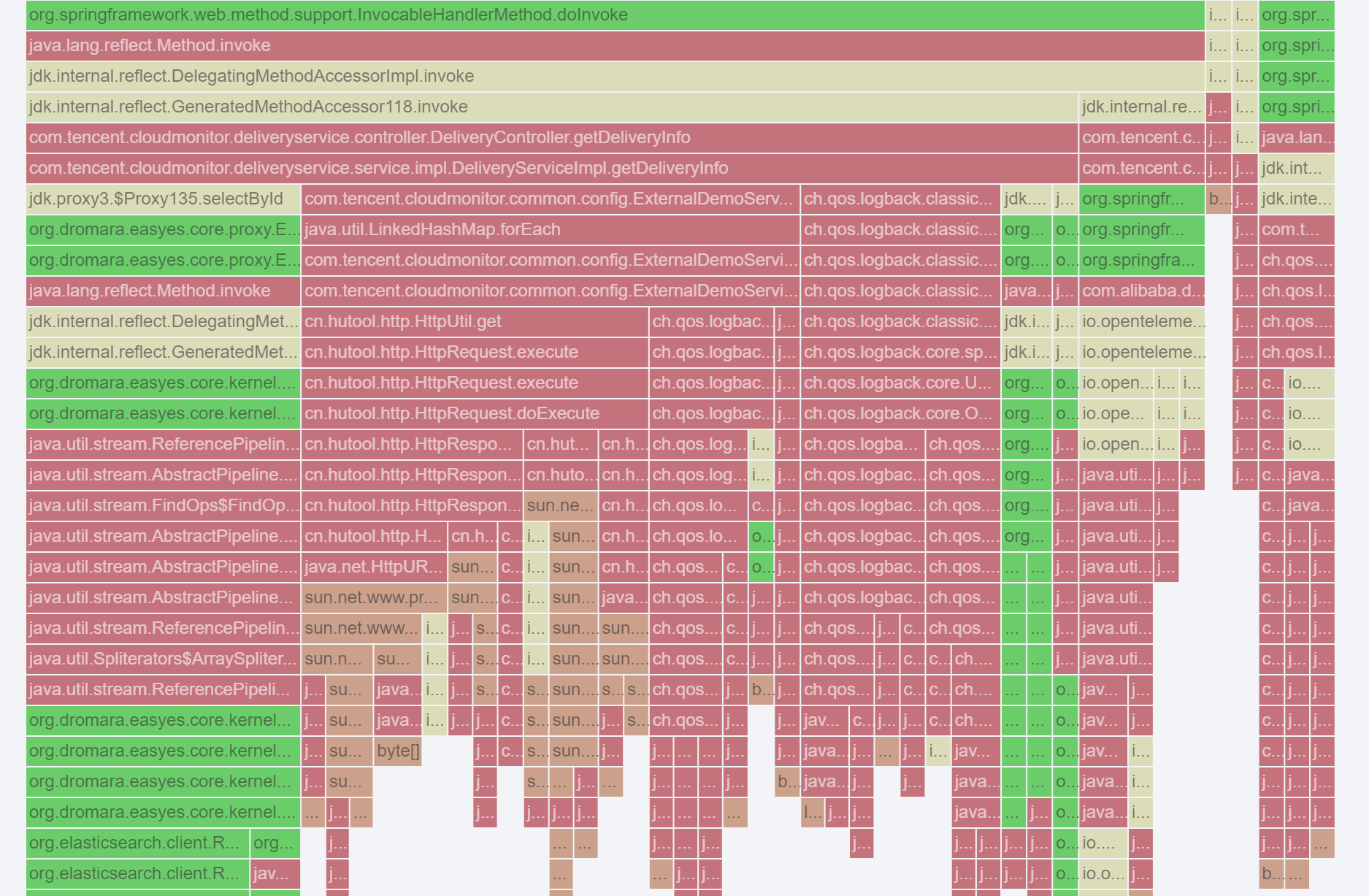
A flame graph is a powerful tool for visualizing program performance data. It is a graph composed of stacked rectangular bars, where each layer of bars represents a function in the function call stack.
Call Graph
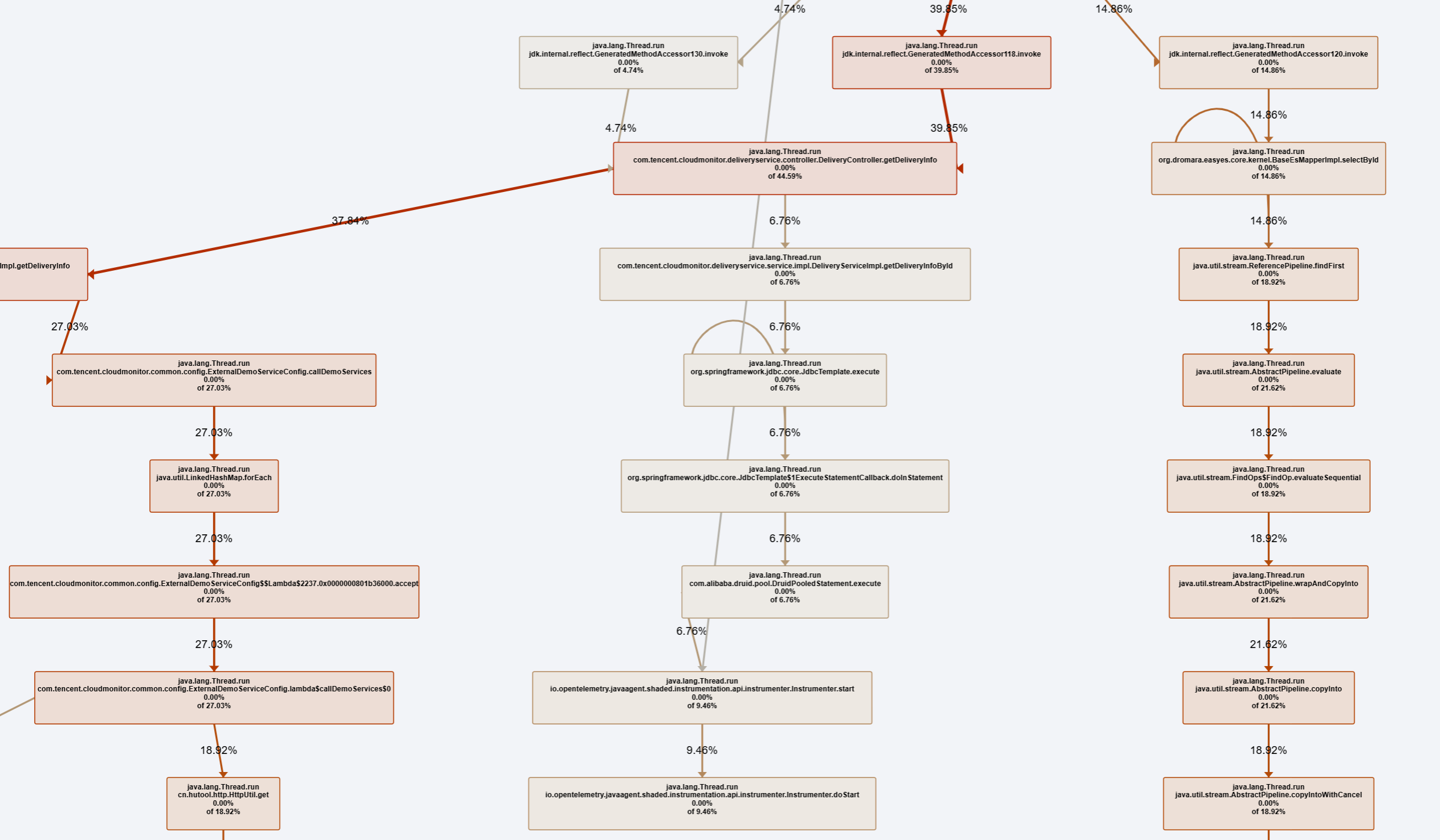
A call graph is a directed graph used to visually display the calling relationships and execution flow between functions in a program. It is quite similar to a flame graph and can also reflect the relative performance cost proportion of each function during the entire program execution process.
Profiling Records
When there are multiple profiling results, the console displays the latest one by default. You can click Profiling Records to view profiling results from other tasks.
Go Application Memory Sampling Analysis
For Go application memory sampling analysis, APM presents the profiling results in two dimensions: Heap and Goroutine. The memory spaces corresponding to these two dimensions are described as follows:
Heap: A memory space shared by multiple goroutines.
Goroutine: A lightweight memory space private to each goroutine.
Among them, the Hot Functions, Flame Graph, and Call Graph features support displaying profiling results from both dimensions in separate tabs. The Analysis Suggestions feature consolidates profiling results from both dimensions into a single tab for display. If no significant bottleneck is detected in a particular dimension, the corresponding performance optimization suggestion is empty.
Flame Graph
In a flame graph, the width of a horizontal bar represents the function's performance overhead, while the vertical direction indicates the depth of the call stack. By observing wide bars, you can quickly locate hot functions for optimization. By examining the vertical direction, you can analyze call relationships to gain a deeper understanding of the execution flow and performance bottlenecks. When a flame graph is analyzed, it is recommended to start with the function at the greatest depth. The deeper the stack, the lower its position appears in the flame graph, which is the location of the 'flame tip' (unlike natural flames, in the flame graphs currently used by APM, the flame points downward). The wider the tip, the greater the performance consumption it represents. Therefore, wide flame tips are often the root cause of performance issues.
When using flame graphs, you can focus on the following two types of metric data:
Total Proportion: Indicates the proportion of performance overhead from the bottom of the function call stack to the current function, including the current function and all its sub-functions. This data reflects the relative importance of the current function and its entire call path during the overall program execution.
Self Proportion: Refers to the performance overhead of the current function itself, excluding the performance overhead of the other functions it calls. This metric helps developers understand the performance overhead of the current function itself, without being affected by the other functions it calls.
When you click a bar in the flame graph, only the bars that lie on its vertical call path within the flame graph are displayed. In this case, this bar can be referred to as the Selected Area, while the area occupied by the entire application process can be referred to as the Overall Area (that is, the topmost root bar). Therefore, both Total Proportion and Self Proportion can be calculated based on either the Selected Area or the Overall Area. Clicking the topmost root bar returns the flame graph to its initial state. In this case, the overall area is equivalent to the selected area.
Call Graph
Call graphs are quite similar to flame graphs, as they also can show the relative proportion of performance overhead for each function during the overall program execution. Unlike flame graphs, when a function has multiple callers, call graphs better illustrate the calling relationships between functions. However, performance overhead cannot be intuitively displayed by the width of bars in a call graph. Therefore, in most scenarios, call graphs are used in conjunction with flame graphs.
Arthas Analysis
Arthas can diagnose application performance without modifying the application code, including viewing the input and output parameters and exceptions of method calls, monitoring method execution time, and obtaining class loading information, thereby significantly improving the efficiency of online issue troubleshooting. The Tencent Cloud enhanced OpenTelemetry Java Agent has built-in Arthas capability. For operations on the Arthas console, see the project homepage.
Thread Analysis
Thread Analysis is a dedicated tab in Application Diagnostics for troubleshooting thread-level issues. It provides a real-time thread snapshot of the current application instance, helping you quickly locate online issues such as thread deadlocks, thread pile-ups (stalls), and hot threads corresponding to CPU spikes, and directly correlate these issues to specific lines of code.
Creating a Collection Task
1. Click Create Collection Task.
2. In the pop-up dialog box, click Confirm.
Analysis Report
After the collection is complete, the console displays the analysis report, which includes the following modules:
Module
Description
Thread list
Displays a list of all current threads in the instance, including key information such as thread name, thread ID, and thread status.
Analyzing Deadlocks
When a deadlock thread exists in the instance, the console displays the threads involved in the deadlock and the lock object relationships on which they are mutually waiting.
Thread statistics
Counts thread quantity based on thread state and thread grouping.
Stack frame statistics
Stack frame statistics merges and aggregates the call stacks of all threads in the current instance, groups threads with identical stack characteristics, and counts the number and proportion of threads in each group.
Thread Pool Analysis
The Thread Pool Analysis feature can display various key metrics of the application's core thread pool, including maximum thread quantity, core thread quantity, active thread quantity, thread pool task quantity, and thread pool size.
Supported Thread Pools
Apache Dubbo 2.7+
Apache Tomcat 7.0+
OkHttp 2.x/3.x/4.x
Metric Details
Maximum thread count: Corresponds to ThreadPoolExecutor.getMaximumPoolSize().
Core thread count: Corresponds to ThreadPoolExecutor.getCorePoolSize().
Active thread count: Corresponds to ThreadPoolExecutor.getActiveCount().
Thread pool size: Corresponds to ThreadPoolExecutor.getPoolSize().
Thread pool task quantity: Corresponds to ThreadPoolExecutor.getQueue().size()
Thread pool utilization: Active thread quantity / Maximum thread quantity * 100%
Connection Pool Analysis
Supported Connection Pools
Apache Druid 1.0+
HikariCP 3.0+
Redisson 3.0+
Jedis 3.0+
Lettuce 5.0+
Apache HttpClient 4.4+
OkHttp 2.x/3.x/4.x
Metric Details
Taking the Druid connection pool as an example, APM collects the following metrics:
Current number of connections: Corresponds to DruidDataSource.getPoolingCount() + DruidDataSource.getActiveCount()
Maximum number of connections: Corresponds to DruidDataSource.getMaxActive()
Active number of connections: Corresponds to DruidDataSource.getActiveCount()
Idle number of connections: Corresponds to DruidDataSource.getPoolingCount()
Connections awaiting: Corresponds to DruidDataSource.getWaitThreadCount().
Note:
For other connection pools, APM collects connection quantity metrics in a similar manner. Due to differences in implementation mechanisms, some connection pools may not report the connections awaiting metric.
Method Execution Analysis
Method execution analysis uses instrumentation to perform line-by-line statistics on the execution time of different stages within a specified method body. This helps you precisely locate performance bottlenecks within a method, identifying exactly which line of code or which sub-call is causing the slowdown.
Creating a Collection Task
1. Click Create Collection Task, and fill in the following information in the pop-up window:
Field
Required
Description
Instance
Automatic
The IP address of the currently selected instance (for example, 10.6.0.156) cannot be modified.
Class Name
Required
The fully qualified class name of the target method, for example, com.test.web.UserController.
Method Name
Required
The target method name, for example, getUser.
Parameter Type
Optional.
When method overloading exists, enter the parameter types separated by commas in order, for example, int, java.lang.String.
Collection Count
Required
The number of collection calls, ranging from 1 - 100 (default: 10).
Max Collection Duration
Required
The maximum wait time for collection, ranging from 10 - 600 seconds (default: 60 seconds).
2. After completing the form, click Confirm to start the collection.
Analysis Results
After the collection is complete, the page displays the line-by-line time consumption analysis for the method:
Field
Description
Analysis record information
The class name, method name, actual number of collections, and collection time are displayed at the top of the page.
Calling Method
The complete method signature (including class name and method name) for each line call within the method body.
Number of rows
The line number of the call in the source code (the entry method itself is displayed as -1).
Timeline
A blue bar chart that intuitively displays the time consumption proportion of each line of code; the longer the bar, the higher the time consumption.
In the result list, the entry method (for example, OrderService.generateOrderInfo) is displayed with the longest blue bar representing its total time consumption. Below it, sub-calls are listed line by line along with their corresponding line numbers and timelines, enabling you to directly locate the code line with the longest execution time.
GC Log Analysis
The GC Log Analysis feature identifies potential risks that may affect application performance based on the GC Log output by the JVM.
Prerequisites
Before using this feature, ensure that JVM has been configured with startup parameters related to GC log printing.
Startup Parameters Related to GC Log Printing
Java 8
Example startup parameters are as follows: -XX:+PrintGCDetails -XX:+PrintGCDateStamps -XX:+PrintGCTimeStamps -XX:+PrintHeapAtGC -Xloggc:gc.log -XX:+UseGCLogFileRotation -XX:GCLogFileSize=20M -XX:NumberOfGCLogFiles=5
Example startup parameters are as follows: -Xlog:gc*:file=gc_%p_%t.log:time,pid:filecount=5,filesize=20M
Alternatively, specify the absolute path for the GC log directly: -Xlog:gc*:file=/path/to/gc.log:time,pid:filecount=5,filesize=20M
Note:
Here, `file` is a required parameter for specifying the GC log file path. For more detailed parameter configurations, see the Java official documentation.
Creating a Collection Task
1. Click Create Collection Task. In the pop-up dialog box, select Data Duration, which represents the time span to look back from the GC log. Then, click Confirm.
2. The total analysis time ranges from a few seconds to about five minutes, depending on the size of the GC log content within the selected data duration. APM can analyze up to 100 MB of GC log data, and any excess portion will be truncated.
Analysis Report
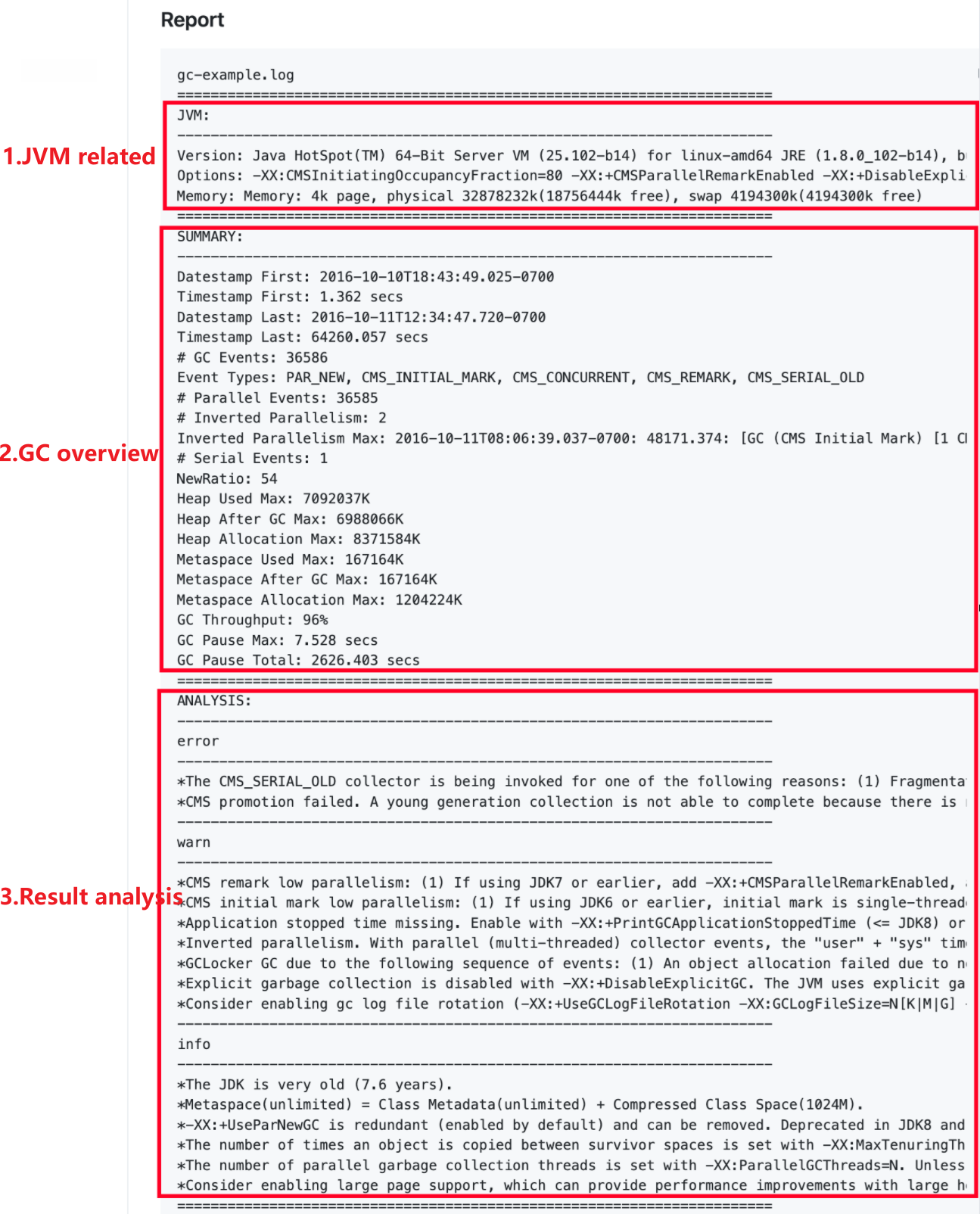
The analysis report contains three parts:
JVM Information: Currently, it is displayed only in JDK 8. It records information such as the JVM version, startup parameters, and system properties.
Summary: Displayed when there are GC behaviors in the selected time period. Pay attention to information such as the log start time, total number of GC events, and GC throughput. GC throughput is an important metric for measuring the performance of Java GCs. You can try different GCs or adjust the related parameters of a GC to obtain a lower GC count and higher GC throughput.
Analysis: Displayed when there are GC behaviors in the selected time period. The analysis result summarizes possible GC issues, provides reasons for the issues, and offers solution suggestions. It is the core content of the analysis report. Focus on the error and warn sections in the analysis result.
Refer to the following analysis report:
Summary
GC Events: 36,586. This value is relatively high. This means that the application may be creating a large number of short-lived objects, potentially leading to frequent garbage collection.
Event Types: During this period, GC events of types PAR_NEW, CMS_INITIAL_MARK, CMS_CONCURRENT, CMS_REMARK, and CMS_SERIAL_OLD are generated.
Parallel Events: 36,585.
Serial Events: 1.
Heap Used Max: 7,092,037 K.
Heap After GC Max: 6,988,066 K. If this value approaches the Heap Used Max, it may indicate inefficient memory usage or a memory leak.
Heap Allocation Max: 8,371,584 K.
Metaspace Used Max: 167,164 K.
Metaspace After GC Max: 167,164 K.
Metaspace Allocation Max: 1,204,224 K.
GC Throughput: 96%. This means that the application spends 96% of its time executing actual business logic and 4% on garbage collection. GC throughput is a metric that measures the performance of Java GCs. It indicates the percentage of time the application is running relative to the total runtime.
GC Pause Max: 7.528 seconds. If the pause time of a single GC is too long, it may affect the response time and delay of the application. For example, if an application needs to complete a transaction within 1000 milliseconds, any GC pause exceeding 1000 milliseconds is unacceptable. Optimization methods may include using concurrent GCs (such as G1 or CMS). These GCs can perform garbage collection while the application is running, thereby reducing the GC pause time.
Analysis
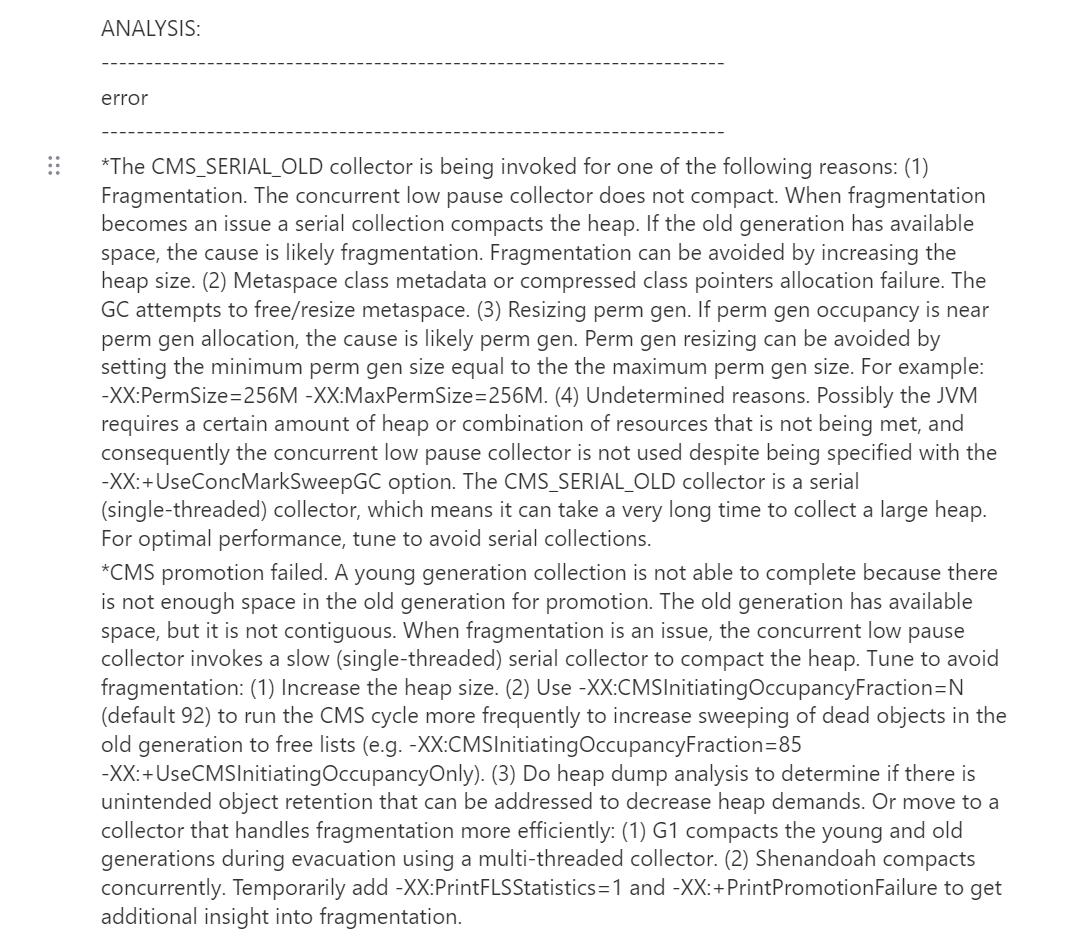
The Analysis summarizes potential GC issues, provides their causes and solutions, and highlights the error and warn sections in the analysis result. For example, the following sample explicitly points out that the CMS_SERIAL_OLD GC runs serially and may require a very long time when reclaiming large memory. It suggests avoiding the use of serial GCs by adjusting JVM parameters. You can tune the JVM based on the analysis results and compare the post-tuning effects using features such as Instance Monitoring in APM.
Runtime Analysis
Runtime analysis includes the following charts:
Function
Description
CPU utilization
Displays the trend of CPU usage. CPU utilization is calculated based on the CPU processing time occupied by the JVM.
Heap memory utilization
Displays the trend of Heap memory usage. Memory utilization = actually used memory / maximum memory requested by the JVM from the operating system.
GC count
Displays the trend of the number of GCs per minute.
Heap memory details
Displays the trend of Heap memory usage.
Thread overview statistics
Counts the trend of thread quantity based on different thread types.